Validation & Results
spectral_galerkin_heat has been checked against three references: the Rosenthal and Eagar–Tsai moving-source solutions in the linear regime, a high-fidelity finite-element (FE) model in the non-linear regime, and a published part-scale scan-strategy study. The first two are agreement checks against a reference. The third is not: there the non-linear physics changes the published result, which is the point of the comparison.
Against analytical solutions (linear regime)
Two moving-source solutions serve as references. Rosenthal’s is closed-form but concentrates the heat input at a point, so it diverges at the beam centre; Eagar–Tsai convolves that point source with a Gaussian matching the beam profile and is evaluated by numerical integration. Both are posed on a semi-infinite medium, so the zero-flux boundaries of the finite cuboid are imposed by the method of images, with one image source along each principal direction.
In the linear case only the Gaussian surface flux contributes to the modal forcing (every other term vanishes), so this comparison tests the reference eigenproblem and the modal integration that sit at the core of the method. The relative \(L^2\) difference between the SG and Eagar–Tsai predictions is below 0.1%.
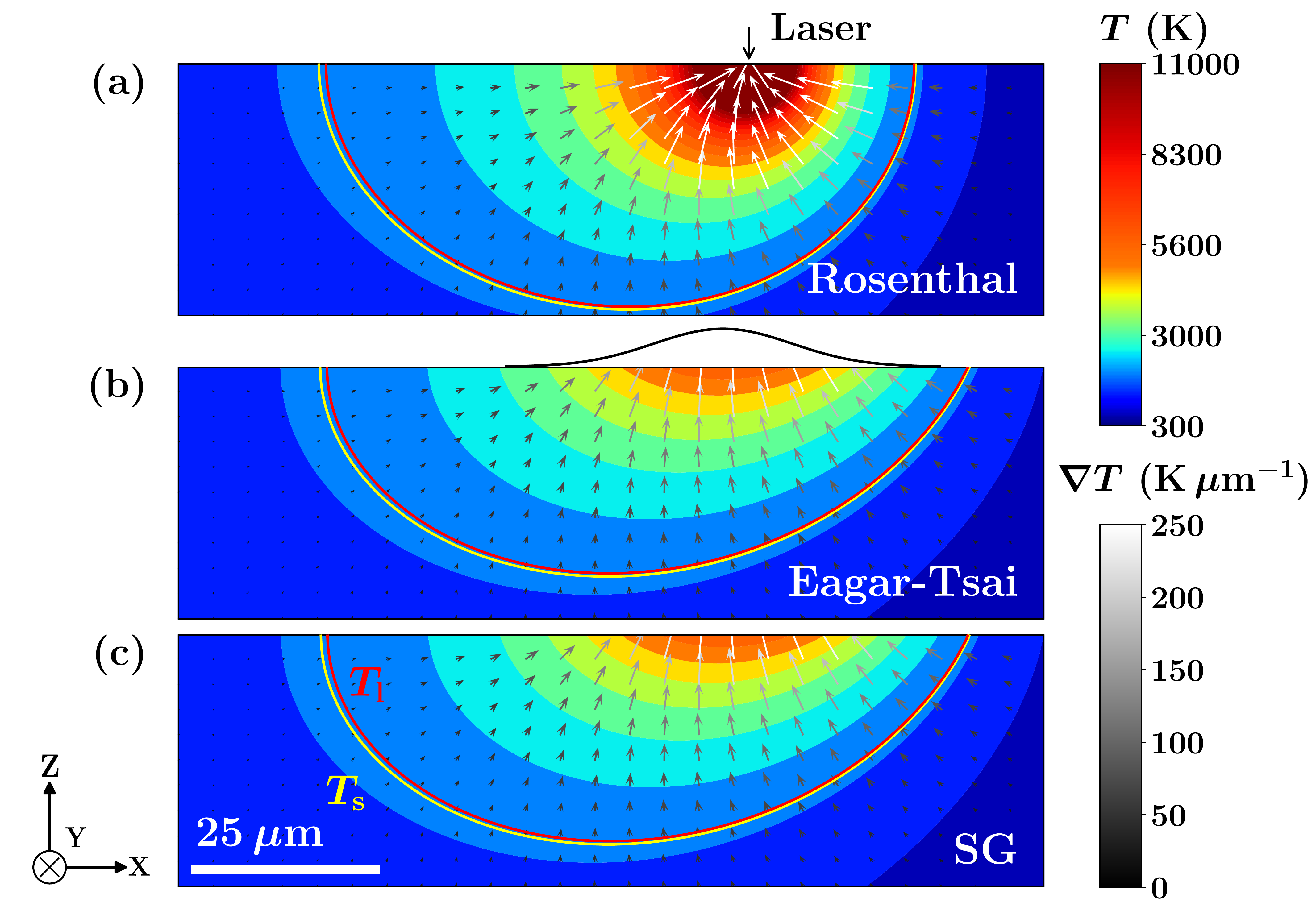
Slices of the temperature field in the \(xz\) plane for the linear case: (a) Rosenthal, (b) Eagar–Tsai, (c) spectral (SG). The yellow and red isolines mark the solidus and liquidus.
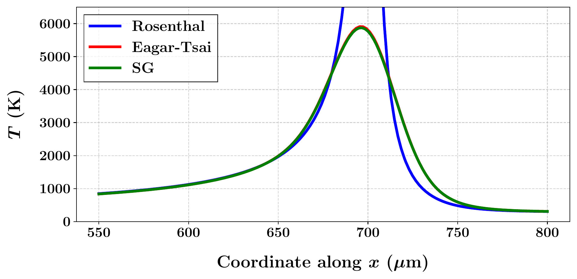
Temperature along the centreline on the top surface, comparing the Rosenthal, Eagar–Tsai and spectral (SG) solutions.
Refining the spectral resolution lowers the relative \(L^2\) error of each run against the finest-resolution SG solution in the same series, a self-convergence check. It drops fast in the in-plane directions (\(x\), \(y\)) and markedly slower in the build direction (\(z\)). The cause is the basis, not the field: every cosine mode has zero derivative at the top surface, so the basis cannot represent the applied flux directly and it enters only through the surface forcing, whose vertical coefficients decay as \(p^{-2}\). The volumetric field then converges as \(N_z^{-3/2}\) and the surface temperature only as \(N_z^{-1}\), which is why the top surface sets the vertical resolution requirement.
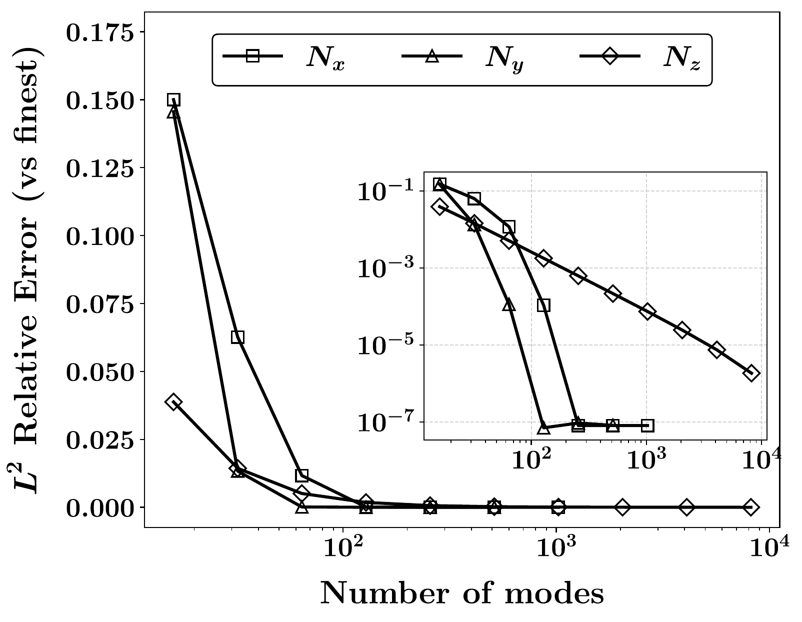
Relative \(L^2\) error between each spectral (SG) run and the finest-resolution SG reference in the same series, versus the number of modes in each direction (log–log).
Against a finite-element reference (non-linear regime)
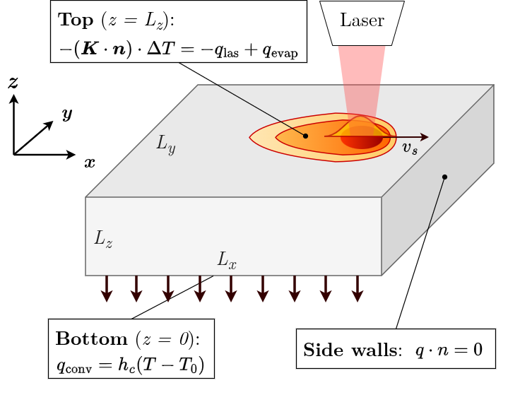
Problem setup: a moving Gaussian laser scans the top surface (\(z = L_z\)) at speed \(v_s\), where the absorbed flux \(q_{\text{las}}\) competes with the evaporative loss \(q_{\text{evap}}\). Convective cooling \(q_{\text{conv}} = h_c(T - T_0)\) is imposed on the bottom surface (\(z = 0\)), and the lateral walls are adiabatic.
Once latent heat of fusion and evaporative cooling enter, no closed form exists, so the spectral solver is compared against an FE model that solves the same governing equations on the same domain with the same properties. The slices show the spectral solver resolving the near-source gradients and the melt-pool shape in agreement with FE. At \(N_x = 256\), \(N_y = 128\), \(N_z = 768\) the relative \(L^2\) difference against FE is 0.67%, and the peak temperature differs by 0.93% (31.3 K).
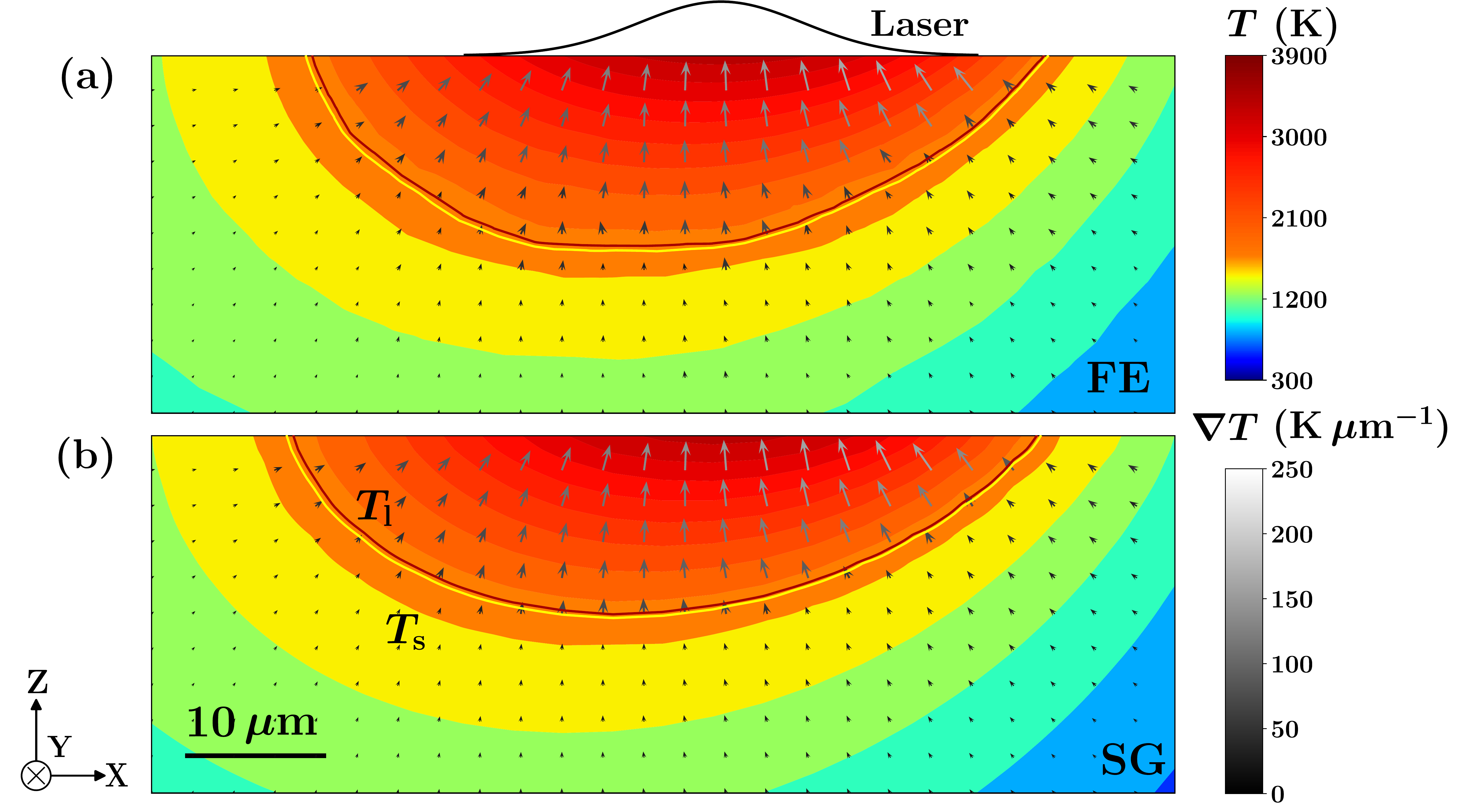
Slices of the temperature field in the \(xz\) plane: (a) finite element (FE), (b) spectral (SG). The yellow and red isolines mark the solidus and liquidus.
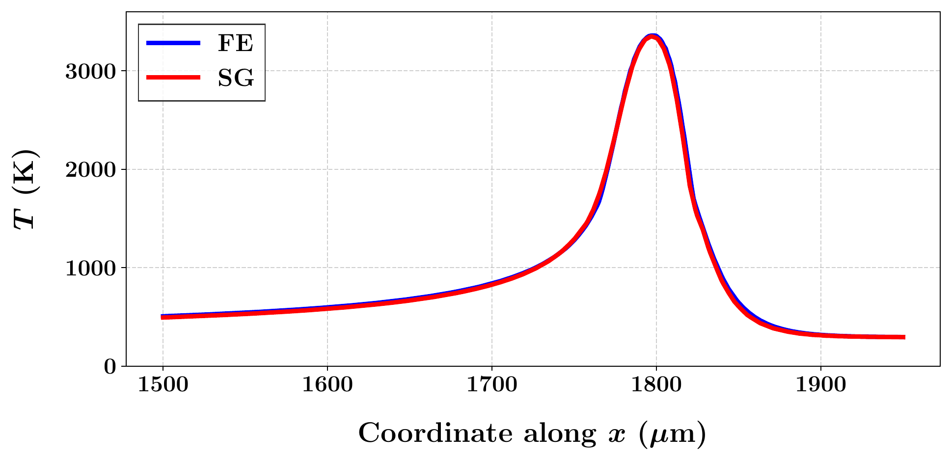
Centreline temperature on the top surface comparing the FE and spectral solutions in the non-linear regime.
Refining the modal resolution again lowers the error against the FE reference, but more slowly than in the linear case, and slowest in \(z\) for the reason given above. The error keeps dropping with further refinement, so a given target accuracy stays reachable: it simply costs more vertical modes.
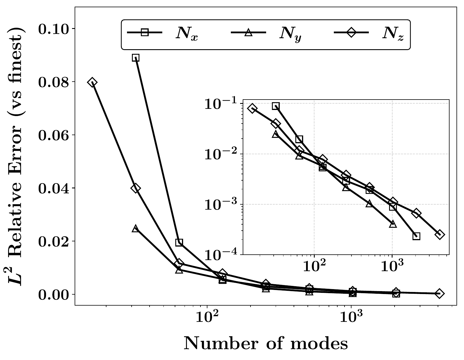
Relative \(L^2\) error between the spectral solver and the FE reference versus the number of modes per direction (log–log).
Performance
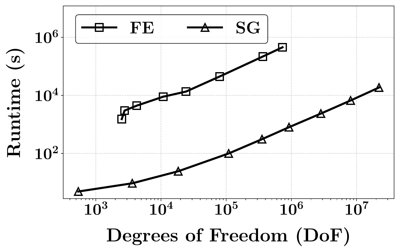
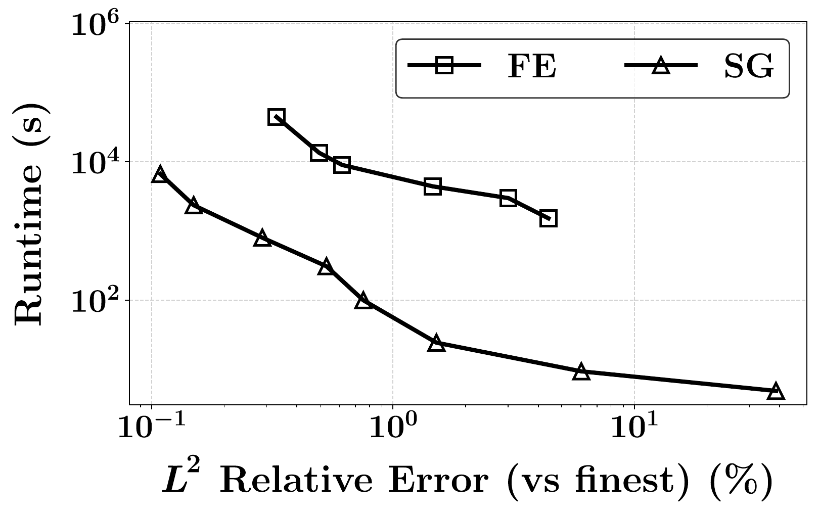
Linear diffusion advances as an element-wise multiply in spectral space, so it is not what sets the cost. With temperature-dependent properties the property correction has to be evaluated over the whole domain, and the spectral transforms that carry it between physical and modal space dominate each step. The complexity is therefore \(\mathcal{O}(N_{\text{vol}} \log N_{\text{vol}})\) in the total number of degrees of freedom. On coarse grids a fixed per-step cost dominates instead and the runtime curve is flat; the asymptotic behaviour appears once the grid is large enough, beyond which the log–log slope is close to 1.
For the non-linear case above, the FE reference needed roughly 189 h on a single core to resolve 2,586,826 degrees of freedom with a 0.6 µm melt-pool mesh. On the same single core, the SG solver resolved a \(256\times128\times768\) grid (25,165,824 degrees of freedom, about an order of magnitude more) in 30.6 h, a factor of 6.2. The same run on a GPU took 0.83 h, a 227-fold reduction relative to the single-core FE baseline.
Application to a literature case study
The solver is applied to the multi-island scan-strategy study of Ramani et al. (2022) for powder-bed fusion of 316L stainless steel, using the same process parameters and scan strategies. That study used a linear finite-difference model. The SG solver first reproduces it directly for validation, then the four strategies are repeated with evaporation and latent heat active and the grid refined to \(N_x = N_y = 1200\), \(N_z = 8\); thermophysical properties are kept constant, since a single-pass simulation in the same regime found temperature-dependence to play a negligible role once evaporation and latent heat are active.
The ranking of the scan strategies is preserved but the absolute numbers are changed: accounting for latent heat and evaporation more than halves both the predicted peak temperature and the thermal-uniformity metric built on it. A linear thermal model can therefore reproduce the qualitative trend while substantially shifting the quantitative thermal state that a process metric is derived from.
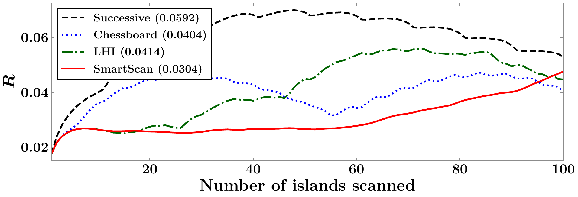
Thermal-uniformity metric \(R(t)\) per scan strategy, from the refined SG run (evaporation and latent heat active). The legend gives each strategy’s mean \(R\).
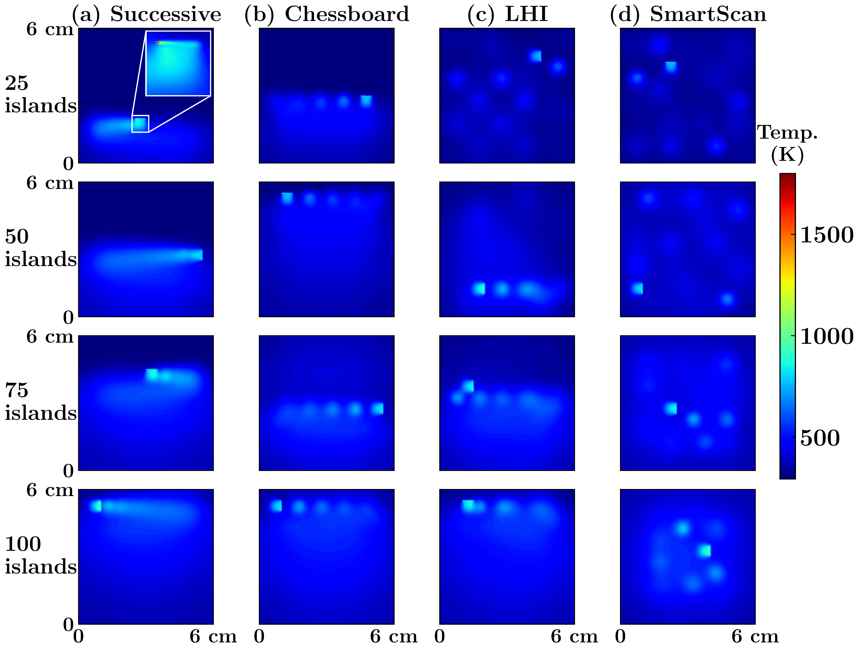
Temperature fields after 25, 50, 75 and 100 islands for each strategy, from the refined SG run.
Reproducibility
The SG-versus-FE timings were measured on a single core of an AMD Ryzen 9 5900X. The CPU/GPU scaling runs used a dual Intel Xeon Gold 5220R (48 cores / 96 threads) and an NVIDIA Quadro RTX 5000 (16 GB). See Examples for the runnable configurations.