Examples

The examples are YAML configurations run through simulations/main.py. They are ordered by increasing complexity: constant properties, then latent heat, then temperature-dependent properties. This page close with library-mode usage. Reading them in order is recommended.

All commands are issued from the repository root with uv:

uv sync   # one-time environment setup

The configurations are in simulations/examples/.

Key concepts

The configuration file

Each example is one YAML file with five top-level sections:

Section	Describes
`simulation`	compute backend, time step `dt`, total `duration`
`domain`	box size `[Lx, Ly, Lz]` and grid `[nx, ny, nz]` (the grid also sets the number of spectral modes)
`material`	density, conductivity, heat capacity, latent heat, and phase-change temperatures
`laser`	beam radius, absorptivity, power, and the path file
`io`	which outputs to write, and where

A value is either a plain number (SI units assumed) or a {value, unit} pair:

dt:
  value: 4.0e-6
  unit: "s"

01_quickstart.yaml is annotated field by field; Configuration Guide lists every key.

The laser path (G-code)

The laser trajectory is a G-code file under simulations/examples/paths/, selected by laser.path.file. The parser reads the subset needed to drive a moving heat source:

Command	Meaning
`G21`, `G90`	millimetre units, absolute coordinates
`G0 X.. Y..`	rapid move, laser off (positioning)
`M3 S<p>` / `M5`	laser on at power `<p>` watts / laser off
`G1 X.. Y.. F<f>`	linear move at feedrate `<f>` (mm/min); sets the scan speed

The quickstart path is a single track scanned at 0.8 m/s with a 200 W beam:

G21 ; mm
G90 ; absolute
G0 X0.0 Y1.25        ; move to start, laser off
M3 S200              ; laser on, 200 W
G1 X9.7 Y1.25 F48000 ; scan +x at 48000 mm/min = 0.8 m/s
M5                   ; laser off

The absorbed power is the beam power (S) times laser.absorptivity. Longer trajectories chain several G0/G1 moves.

1. Quickstart

01_quickstart.yaml scans a single laser track over a coarse cuboid with constant material properties. Latent heat and surface convection are disabled, leaving evaporative cooling as the only non-linear surface flux. The run takes about a minute on one CPU core. Its YAML is annotated field by field and serves as the configuration reference.

uv run python simulations/main.py simulations/examples/01_quickstart.yaml

Results are written to out/<timestamp>_quickstart/:

profiles/ — temperature along \(x\), \(y\), \(z\) through the laser spot (text).
fields/ — the final volume field, readable in ParaView through the .xmf file.
slices/ — the cross-section image configured by io.slice_planes.
logs/simulation.log — per-step metrics (T_surface_max, laser power).

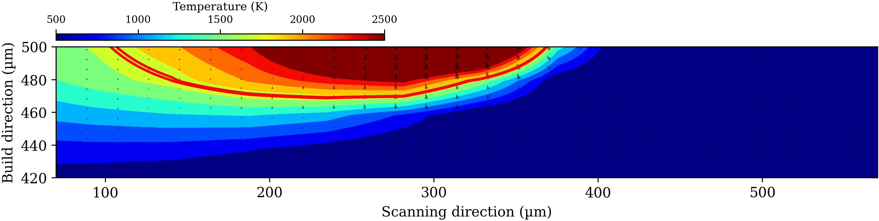
Longitudinal melt-pool section, example 01 — Longitudinal (\(xz\), normal \(y\)) section through the laser spot at the end of the run. The red contour marks the solidus/liquidus.

2. Single track with latent heat

02_single_track.yaml adds the two effects that example 1 omits: latent heat of fusion (L_f) and bottom-face convection (h_conv_bottom). Properties remain constant, obtained by evaluating the temperature-dependent 316L polynomials at \(T_0 = 293\) K. The domain is small with a fine \(z\)-grid (\(\Delta z \approx 1.25\ \mu\text{m}\)) so the narrow 316L mushy zone is resolved. The run takes a few minutes on one CPU core.

Note

The 316L thermophysical properties used in these examples (\(\rho\), \(k\), \(c_p\), with separate solid and liquid branches) are taken from Chadwick et al., Acta Materialia 282 (2025) 120482, doi:10.1016/j.actamat.2024.120482.

uv run python simulations/main.py simulations/examples/02_single_track.yaml

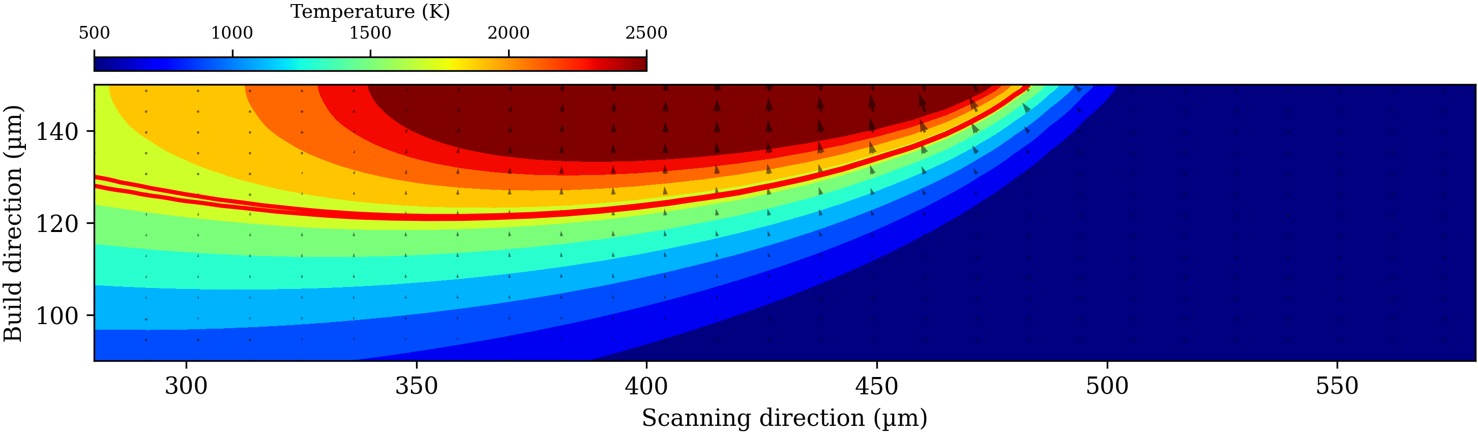
Longitudinal melt-pool section, example 02 — Melt-pool section for the single track. The two red contours are the solidus and liquidus.

3. Temperature-dependent properties

03_nonlinear_tdep.yaml lets the conductivity, density and specific heat vary with temperature (solid and liquid expression branches blended by the liquid fraction), making the problem non-linear. Each step is solved by a Picard iteration that also resolves the property correction (see Theory & Physics):

max_picard_iter — iteration cap per step (80 here).
picard_omega — relaxation factor; larger values converge faster until the iteration destabilises (0.31 is near the limit for this case).

uv run python simulations/main.py simulations/examples/03_nonlinear_tdep.yaml

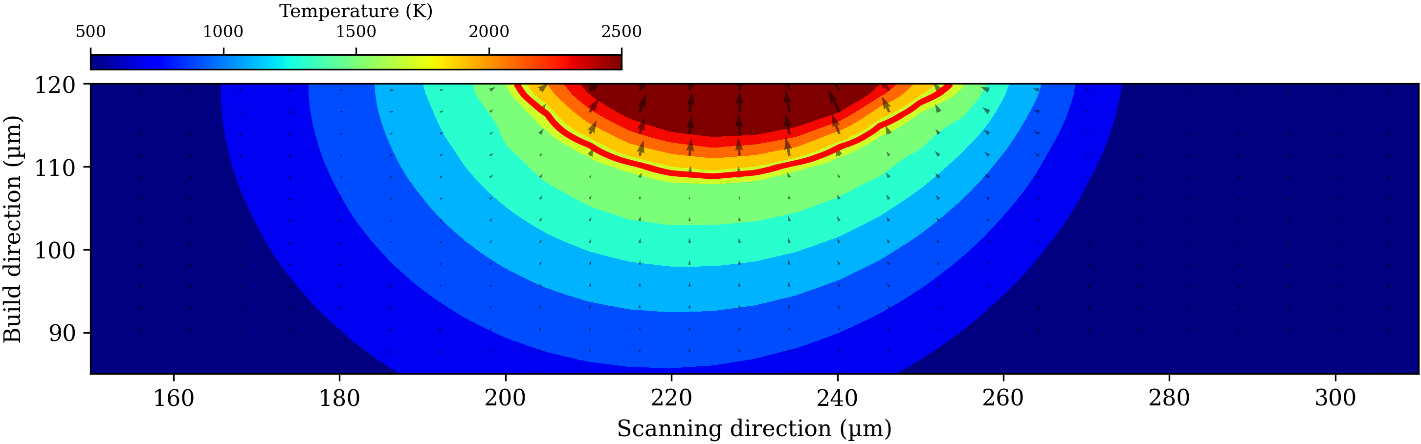
Conduction-mode melt pool, example 03 — Melt-pool section for the temperature-dependent run. The red line marks the solidus/liquidus.

This is a reduced-grid version of the finite-element comparison case.

4. Library mode

The solver can be driven directly from Python rather than the CLI. An external script builds a SimulationContext and calls solver.step(...) in a loop, which is useful when embedding the solver in a larger codebase. Nothing is written to disk.

Installing as a library. To import spectral_galerkin_heat from a project outside this repository, install it as an editable package into your environment:

uv pip install -e /path/to/spectral_galerkin_heat    # or: pip install -e /path/to/spectral_galerkin_heat

Or declare it as an editable source in another uv project’s pyproject.toml:

[project]
dependencies = ["spectral_galerkin_heat"]

[tool.uv.sources]
spectral_galerkin_heat = { path = "/path/to/spectral_galerkin_heat", editable = true }

Either way the import name is spectral_galerkin_heat, and edits to the source take effect without reinstalling. The full runnable script is orchestrator.py:

uv run python simulations/examples/orchestrator.py

from spectral_galerkin_heat.core.parameters import SimulationContext
from spectral_galerkin_heat.solvers.spectral import SpectralSolver
from spectral_galerkin_heat.backends import NumpyBackend

# 1. Configuration as a plain dictionary
config = {
    "simulation": {"backend": "cpu", "dt": 6e-6, "duration": 6e-5},
    "domain": {"size": [0.01, 0.005, 0.0025], "mesh": [64, 32, 16]},
    "material": {"rho": 7957.5, "k": 13.851, "Cp": 497.89, "name": "316L"},  # reference 316L values
    "laser": {"radius": 60.0e-6, "absorptivity": 0.30, "power_nominal": 200.0,
              "path": {"type": "gcode", "file": "linear_track.gcode"}},
    "io": {},   # empty: the IOManager is not used
}

# 2. Build the context. config_dir must point to the directory holding the
#    paths/ subfolder with the G-code (use an absolute path when running elsewhere).
context = SimulationContext.from_dict(config, config_dir="simulations/examples")

# 3. Instantiate and initialise the solver
solver = SpectralSolver(NumpyBackend())   # get_backend("cupy") for GPU
state = solver.initialize(context)

# 4. Time loop
t, dt, t_end = 0.0, context.num.dt, context.num.t_end
while t < t_end:
    state, metrics = solver.step(t, dt)
    t += dt
    print(f"t = {t:.4e} s | T_max = {metrics.get('T_surface_max'):.1f} K")